What is a sensor and how does sensing fit with Machine Learning ? This is a common question that I think arise out of the fact that our fields are becoming too specific thereby attenuating our common sense of what the big picture entails. Be forewarned, the following brief exposition will be making numerous shortcuts and abuse of notation.
Everything starts with the simple notion that what you see is what you get:
x = x
In other words, on one side, you have x and on the other you "sense" x. This picture applies directly to what we call direct imaging: if you want to image something, you have to just sample it. A more mathy expression for this process is the simple:
x = I x
where I is the identity (yes, let's talk about matrices or operators when the explanation requires it.) Let us note that sometimes, when we remove certain rows from I by applying a restriction operator R, then we are undersampling. Reconstructing the full x from that subsampled version (RIx) is called interpolation or inpainting. Let us call IN that inpainting operator so that we have:
x = IN (R(Ix))

So far so good. Let us also note that in optics we generally do the following:
x = (BA) x
(BA) generally represents the lenses of the camera. In other words, the engineering behind lens design (using tools like Zemax) is geared towards designing BA (also called the PSF) to be as close as possible to I, the identity. The sensor or the measurement process obtains (BA)x. Both A and B are linear operators. The process is actually a little more complex see [1].

Then there is the case of indirect imaging as attempted since the early 1960s with coded aperture for instance.
x = L(Ax)
L and A are linear operators. The sensors can only measure Ax (not x) but you are a matrix multiplication away from getting x back. Famous examples include coded aperture for X-ray imaging for orbital observatories, but also CT and MRI. Encryption also fits that model.

Credit: Rice University
With compressive sensing, things get a little more complicated, it is indirect imaging but with a twist. There we have
x = N(Ax) or even x = N(A(Bx))
with A or A and B are linear operators, x is sparse (or compressible) in the canonical basis or in some other bases, N is a nonlinear operator. Here, as in indirect imaging, what is sensed is Ax or A(Bx). The difference between this new approach and traditional indirect imaging lies the nonlinearity of the reconstruction operator N. In compressive sensing, we seek a rectangular A (subsampling) and the nonlinearity of the N comes from the fact that we seek only sparse x's. Historically, N was initially tied to linear convex programming or greedy methods, but there are other different approaches such as IHT and eventually AMP. Additional insight can be found in [2].
Muthu (see [3]) points out that there ought to be other quantities we could extract from a linear sensing mechanism so that instead of:
x = N(Ax)
we ought to look at:
Hx = N(Ax)
The sensor obtains Ax, N is a nonlinear reconstruction solver of sorts that reconstruct Hx which is an hopefully important feature of x (in compressive sensing, that feature is the sparsity pattern of x). Instead of the full reconstruction, we aim at detecting items of interest. In optics we sometimes talk about task specific imagers or detection of features in manifold signal processing, in MRI, we call it fingerprinting while in Theoretical Computer Science, we are concerned about the statistics of x since in the streaming model, we cannot even store x. There the process goes by the name of Heavy Hitters and related algorithms. It looks like homomorphic encryption would fit that model. One could also argue that current conventional direct imaging also falls in that category. (see [1])
Now let us go further by making the first sensing operator a nonlinear one. This is the approach that is typically seen in nonlinear compressive sensing and also in machine learning. There we have:
x = N2(N1(x))

x = N4(N3(N2(N1(x))))
This sort of very successful construct is known as autoencoders in deep learning. Each operator N is nonlinear. A specific choice of regularization for the layers and nodes can even make it look like a compressive sensing approach. In this case. we talk about sparse autoencoders, i.e. roughly speaking , there is sparse set of weights for every images that are part of the training set on which the neural network was trained. In traditional sensing, there are also natural nonlinear sampling schemes such as the one introduced by quantization (see Petros' resource on Quantization), or FROG or simply those found in phase retrieval problems.
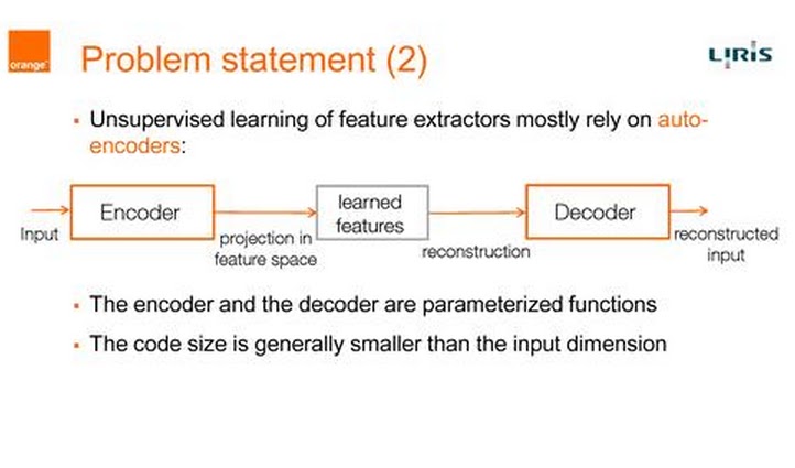
From " Spatio-Temporal Convolutional Sparse Auto-Encoder for Sequence Classification" by Moez Baccouche,
And then there is the traditional area of Machine Learning that does classification:
Hx = N4(N3(N2(N1(x))))
where Hx represents whether x belongs to a class (+1/-1).
As we have seen recently, the connection between Compressive Sensing and Machine Learning, stems in large part in the nonlinearities involved in the sampling stage and specifically how to grab the features of interest. Can we be guided on the preferable nonlinearities ? When one comes back to a linear case, there are interesting information that might eventually be useful for designing nonlinearities in the sampling system, from [4]:
As we have seen recently, the connection between Compressive Sensing and Machine Learning, stems in large part in the nonlinearities involved in the sampling stage and specifically how to grab the features of interest. Can we be guided on the preferable nonlinearities ? When one comes back to a linear case, there are interesting information that might eventually be useful for designing nonlinearities in the sampling system, from [4]:
We show that the suggested instance optimality is equivalent to a generalized null space property of M and discuss possible relations with generalized restricted isometry properties.
There are also other lessons to be learned from [5] but this time it involves low rank issues and some condition on the nonlinearity. We are just at the beginning of seeing these two fields merging.
[1] Let us note that this is not entirely true in conventional imaging, a 2D scene is transformed into a 2D scene whereas a 3D scene is transformed into a 2D scene. So AB is not really the identity but some sort of the projection of it Let us further note that in conventional direct imaging, things are really more complicated as AB is really two nonlinear operators that include the nonlinearities of the FPA, quantization issues and compression (JPEG, ...). This is one the reason why Mark Neifeld tells us that we are already using compressive systems in a talk entitled Adaptation for Task-Specific Compressive Imaging


[2] One should note that the rapid convergence of some of these algorithms makes one think that they could be parallel to neural networks. There are conditions on A, x, N although those are better acknowledged than in the direct imaging case. But there is really no restriction due to the concept of sparsity, indeed other solvers N using l_infty, l_p and other norms as regularizers can find a signal with a certain structure within the set of signals that were not destroyed by A (or A(B.)). With an underdetermined system (rectangular A), what we are saying in essence is that by performing the measurement Ax, we are not losing information on x.
Compressed Functional Sensing. Streaming and compressed sensing brought two groups of researchers (CS and signal processing) together on common problems of what is the minimal amount of data to be sensed or captured or stored, so data sources can be reconstructed, at least approximately. This has been a productive development for research with fundamental insights into geometry of high dimensional spaces as well as the Uncertainty Principle. In addition, Engineering and Industry has been impacted significantly with analog to information paradigm. This is however just the beginning. We need to extend compressed sensing to functional sensing, where we sense only what is appropriate to compute different function (rather than simply reconstructing) and furthermore, extend the theory to massively distributed and continual framework to be truly useful for new massive data applications above.
We propose a theoretical study of the conditions guaranteeing that a decoder will obtain an optimal signal recovery from an underdetermined set of linear measurements. This special type of performance guarantee is termed instance optimality and is typically related with certain properties of the dimensionality-reducing matrix M. Our work extends traditional results in sparse recovery, where instance optimality is expressed with respect to the set of sparse vectors, by replac- ing this set with an arbitrary finite union of subspaces. We show that the suggested instance optimality is equivalent to a generalized null space property of M and discuss possible relations with generalized restricted isometry properties.
 Liked this entry ? subscribe to Nuit Blanche's feed, there's more where that came from. You can also subscribe to Nuit Blanche by Email, explore the Big Picture in Compressive Sensing or the Matrix Factorization Jungle and join the conversations on compressive sensing, advanced matrix factorization and calibration issues on Linkedin.
No comments:
Post a Comment